Machine Learning
A machine-Learning Learning notes
Supervised learning
Linear regression
model
\[ f_{\omega,b}(x) = wx+b \]
change the w and b to optimize the algorithm.
Cost function
Used to evaluate the model. The goal is to use cost function to minimize it and to find the best parameters for the model.
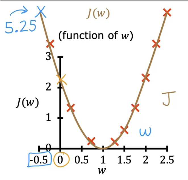
used for linear regression is \[ J(\omega,b) = \frac{1}{2m}\sum_{i=1}^{m}(f_{\omega,b}(x^{(i)})-y^{(i)})^2 \] It's related with w and b
Graph when J is only related to w:
Gradient descent
In a 3D plot which choose w,b as the ground,J(w,b)as the hight.To find the best w,b it needs to go down from a "hill" to a "valley". You look around and go step by step from the hill untill can't go down any further, that's a valley.
algorithm
\[ w=w-\alpha \frac{\partial}{\partial w} J(w, b) \] \[ b=b-\alpha \frac{\partial}{\partial b} J(w, b) \]
\(\alpha\) means "Learning rate", which controls how largh you take for each step downhill.
You need to update w and b simultaneously, the correct method are as follows: \[ \begin{aligned} &t m p_{-} w=w-\alpha \frac{\partial}{\partial w} J(w, b) \\ &{tmp_{-}b=b-\alpha \frac{\partial}{\partial b} J\left(w,b\right)} \\ &w=t m p_{-} w\\ &b=tmp_{-}b \end{aligned} \] Repeat doing this untile w and b convergence.
Why use derivative?
The learning rate is always positive,so if the derivative is negative, to make the J(w,b) smaller you need to increase w. If the derivative is positive, you need to decreate w.
The cost function usually shape like a bowl, so it only have one minimum point.
Multiple Linear regression
\(\mathrm{x}_j\) = \(j^{\text {th }}\) feature
\(\overrightarrow{\mathrm{x}}^{(i)}\) = features of \(i^{\text {th }}\) training example, this is a vector
\(\mathrm{X}_j^{(i)}\) = value of feature j in \(i^{\text {th }}\) training example
Model:
\[ f_{w, b}(x)=w_1 x_1+w_2 x_2+\cdots+w_n x_n+b \]
\(\vec{\omega}=\left[\begin{array}{lllll}w_1 & w_2 & w_3 & \ldots & w_n\end{array}\right]\)
It can be rewritten as:
\(f_{\overrightarrow{\mathrm{w}}, b}(\overrightarrow{\mathrm{x}})=\overrightarrow{\mathrm{w}} \cdot \overrightarrow{\mathrm{x}}+b\)
Vectorization
overall: use numpy as much as possible to make the program run faster.
Without vectorization you need to use for loop to calculate f
With vectorization you can use np.dot(w,x) to get the result.
Multiple Gradient descent
Repeat{
\(\left.w_1=w_1-\alpha \frac{1}{m} \sum_{i=1}^m\left(f_{\overrightarrow{\mathrm{w}}, b}\left(\overrightarrow{\mathrm{x}}^{(i)}\right)-y^{(i)}\right) x_1^{(i)}\right)\)
=>\(\frac{\partial}{\partial w_1} J(\overrightarrow{\mathrm{w}}, b)\)
\(\vdots\)
\(w_n=w_n-\alpha \frac{1}{m} \sum_{i=1}^m\left(f_{\overrightarrow{\mathrm{w}}, b}\left(\overrightarrow{\mathrm{x}}^{(i)}\right)-y^{(i)}\right) x_n^{(i)}\)
\(b=b-\alpha \frac{1}{m} \sum_{i=1}^m\left(f_{\overrightarrow{\mathrm{w}}, b}\left(\overrightarrow{\mathrm{x}}^{(i)}\right)-y^{(i)}\right)\)
simultaneously update \(w_j(\) for \(j=1, \cdots, n)\) and \(b\)
}
Feature scaling
Choose proper w1,w2...can make gradient descent faster.
Logistic regression
use sigmoid function to make classifition.
Sigmoid function:
\(g(z)=\frac{1}{1+e^{-z}} \quad 0<g(z)<1\)
Logistic regression model: \[ z=\overrightarrow{\mathrm{w}} \cdot \overrightarrow{\mathrm{x}}+b \\ g(z)=\frac{1}{1+e^{-z}} \]
Decision boundary
choose a threshold to determin whether \(\hat y\) is 0 or 1.
Normally use when \(z=\overrightarrow{\mathrm{w}} \cdot \overrightarrow{\mathrm{x}}+b=0\) when it's a linear situation.
When it's a non-linear situation, use this one \(z=x_1^2+x_2^2-1=0\)
Cost/Lost function
Previous: \(J(\overrightarrow{\mathrm{w}}, b)=\frac{1}{m} \sum_{i=1}^m \frac{1}{2}\left(f_{\overrightarrow{\mathrm{w}}, b}\left(\overrightarrow{\mathrm{x}}^{(i)}\right)-y^{(i)}\right)^2\) squared error.
It's cost function is a non-convex, so need a new function.
new version: \[ L\left(f_{\overrightarrow{\mathrm{w}}, b}\left(\overrightarrow{\mathrm{x}}^{(i)}\right), y^{(i)}\right)=\left\{\begin{aligned} -\log \left(f_{\overrightarrow{\mathrm{w}}, b}\left(\overrightarrow{\mathrm{x}}^{(i)}\right)\right) & \text { if } y^{(i)}=1 \\ -\log \left(1-f_{\overrightarrow{\mathrm{w}}, b}\left(\overrightarrow{\mathrm{x}}^{(i)}\right)\right) & \text { if } y^{(i)}=0 \end{aligned}\right. \]

simplified version: \[ L\left(f_{\overrightarrow{\mathrm{w}}, b}\left(\overrightarrow{\mathrm{x}}^{(i)}\right), y^{(i)}\right)=-y^{(i)} \log \left(f_{\overrightarrow{\mathrm{w}}, b}\left(\overrightarrow{\mathrm{x}}^{(i)}\right)\right)-\left(1-y^{(i)}\right) \log \left(1-f_{\overrightarrow{\mathrm{w}}, b}\left(\overrightarrow{\mathrm{x}}^{(i)}\right)\right) \] It's cost function: \[ J(\mathbf{w}, b)=\frac{1}{m} \sum_{i=0}^{m-1}\left[\operatorname{loss}\left(f_{\mathbf{w}, b}\left(\mathbf{x}^{(i)}\right), y^{(i)}\right)\right] \]
1 | def compute_cost_logistic(X, y, w, b): |
overfitting
- Underfit:the model doesn't fit the training set well.(high bias in prediction result)
- Overfit : the model fits the training set extremely well.(high variance in result, small change cause huge difference)
How to deal with it?
- collect more training examples
- Reduce features to use
- reduce the size of parameters(regularization)
Gradient decent
repeat until convergence: { \[ \begin{aligned} &b:=b-\alpha \frac{\partial J(\mathbf{w}, b)}{\partial b} \\ &w_j:=w_j-\alpha \frac{\partial J(\mathbf{w}, b)}{\partial w_j} \quad \text { for } \mathrm{j}:=0 . . \mathrm{n}-1 \end{aligned} \] } \[ \begin{gathered} \frac{\partial J(\mathbf{w}, b)}{\partial b}=\frac{1}{m} \sum_{i=0}^{m-1}\left(f_{\mathbf{w}, b}\left(\mathbf{x}^{(i)}\right)-\mathbf{y}^{(i)}\right) \\ \frac{\partial J(\mathbf{w}, b)}{\partial w_j}=\frac{1}{m} \sum_{i=0}^{m-1}\left(f_{\mathbf{w}, b}\left(\mathbf{x}^{(i)}\right)-\mathbf{y}^{(i)}\right) x_j^{(i)} \end{gathered} \]
1 | def compute_gradient_logistic(X, y, w, b): |
1 | def gradient_descent(X, y, w_in, b_in, cost_function, gradient_function, alpha, num_iters, lambda_): |
Decision tree
A predict which features are discrete values.
Questions about the algorithm:
- How to choose parameters?
- Maximize purity
- When to stop splitting
- When a node is 100% one class
- When splitting a node will result in the tree exceeding a maximum depth
- When improvements in purity score are below a threshold
use Entropy to measure purity

\(\begin{aligned} H\left(p_1\right) &=-p_1 \log _2\left(p_1\right)-p_0 \log _2\left(p_0\right) \\ &=-p_1 \log _2\left(p_1\right)-\left(1-p_1\right) \log _2\left(1-p_1\right) \end{aligned}\)
Neural Networks
Neural Network Model
activation function:\(a=f(x)=\frac{1}{1+e^{-(w x+b)}}\)
If a vector X begin input into the first layer which consists three neurons.
Each neuron will return \(a_1=g(\overrightarrow{\mathrm{w}} \cdot \overrightarrow{\mathrm{x}}+b)*weight\) and composits a vector of three numbers, which is the output of this layer.
\(w_1^{\text {[1] }}\) denotes the first layer's first w.
Mutiple layers neural networks
Notation:
\(a_j^{[l]}=g\left(\vec{w}_j^{[l]} \cdot \vec{a}^{[l-1]}+b_j^{[l]}\right)\)

Forward propagation

specific calculation:
\(x=n p \cdot \operatorname{array}([200,17])\)
\(a_1^{[1]}=g\left(\overrightarrow{\mathrm{w}}_1^{[1]} \cdot \overrightarrow{\mathrm{x}}+b_1^{[1]}\right)\)
w1_1 \(=\) np. array \(([1,2])\) b1_1 \(=\) np. \(\operatorname{array}([-1])\) \(z 11=n p \cdot \operatorname{dot}(w 11, x)+b 11\) a1_1 = sigmoid \(\left(z 1_{-1}\right)\)
and then a1 = np. array( [a1_1,a1_2,a1_3]
Training a neural network
- specify how to compute output
- specify loss and cost
- Train to minimize lost
Create model
use sequence and dense func
Train model
repeat { \[ \begin{aligned} &w_j^{[l]}=w_j^{[l]}-\alpha \frac{\partial}{\partial w_j} J(\overrightarrow{\mathrm{w}}, b) \\ &b_j^{[l]}=b_j^{[l]}-\alpha \frac{\partial}{\partial b j} J(\overrightarrow{\mathrm{w}}, b) \end{aligned} \] \[ \text { \} } \]
model.fit(X,y,epochs=100)
Activation functions
Linear activation function \(g(z)=z\)
Sigmoid \(g(z)=\frac{1}{1+e^{-z}}\)
ReLU \(g(z)=\max (0, z)\)

How to choose?
output layer:
Binary cassification: Signoid
Regression:Linear activation
Regression with all positive:ReLU
Hidden layer
in hidden layer mostly ReLU
Multiclass Classification
Softmax regression
\(z_1=\overrightarrow{\mathrm{w}}_1 \cdot \overrightarrow{\mathrm{x}}+b_1\)
\(a_1=\frac{e^{z_1}}{e^{z_1}+e^{z_2}+e^{z_3}+e^{z_4}}\) \[ z_j=\overrightarrow{\mathrm{w}}_j \cdot \overrightarrow{\mathrm{x}}+b_j \quad \mathrm{j}=1, \ldots, \mathrm{N} \]
\[ a_j=\frac{e^{z_j}}{\sum_{k=1}^N e^{z_k}}=\mathrm{P}(\mathrm{y}=j \mid \overrightarrow{\mathrm{x}}) \]
Cost
\[ a_N=\frac{e^{z_N}}{e^{z_1}+e^{z_2}+\cdots+e^{z_N}}=P(y=N \mid \overrightarrow{\mathrm{x}}) \]
\[ \operatorname{loss}\left(a_1, \ldots, a_N, y\right)=\left\{\begin{array}{lc} -\log a_1 & \text { if } y=1 \\ -\log a_2 & \text { if } y=2 \\ & \vdots \\ -\log a_N & \text { if } y=N \end{array}\right. \]
Programming
1 | Dense(units=10,activation='softmax')#output layer |
Better way(recommended):
To make it more numerically accurate.
From \(\operatorname{loss}=-y \log (a)-(1-y) \log (1-a)\)
to \(\operatorname{loss}=-y \log \left(\frac{1}{1+e^{-z}}\right)-(1-y) \log \left(1-\frac{1}{1+e^{-z}}\right)\)
1 | Dense(units=10,activation='linear') |
Optimization and Diagnosing
Adam algorithm
Adaptive Moment estimation
automatically change alpha while doing learning.Has a lot of alpha for different parameters.
1 | compile(tf.keras.optimizers.Adam(learning_rate=1e-3)) |
Layer types
Dense Layer
output is a function of all the activation function result
Convolutional Layer
Each neuron only looks at part of the previous layer's output
Unsupervised Learning
PCA(principle component analysis)
theoretical part
It's propose is to reduce dimension of input data. Suppose we have sample X with n dimensions \(X=\left\{x_0, x_1, \ldots, x_m\right\}\) and we want to have a transformation \(y=P x\) in which P is a matrix. Then we get some data Y with k dimensions \(Y=\left\{y_0, y_1, \ldots, y_m\right\}\) .
preprocessing data
normolize input data by subtracting their mean of each column.
Do the PCA as follows:
we need to make sure these two laws of PCA:
- After reducing, each of the dimensions should be independent, which means every axis are orthogonal after PCA.
- maximize the variance of each dimensions, which means keeping the original data as much as possible.
First we can denote the covariance matrix after transportation as \(B_{k \times k}=\frac{1}{m} Y Y^T\) , to make each dimensions independent B should be a diagonal matrix, which means it's all 0 except for it's diagonal.
Let's substitute this equation \(y=P x\) into the equation \(B_{k \times k}=\frac{1}{m} Y Y^T\) and get: \[ B_{k \times k}=\frac{1}{m} Y Y^T=\frac{1}{m} P X(P X)^T=P \frac{1}{m} X X^T P^T=P_{k \times n} C_{n \times n} P_{n \times k}^T \] in which \(C_{n \times n}=\frac{1}{m} X X^T\) is the covariance matrix of training data.
Use eigenvalue decomposition on C and get \(D_{n \times n}=Q_{n \times n} C_{n \times n} Q_{n \times n}^T\) and D is a diagonal matrix.
So we can know P is a matrix composed by k-th big eigenvectors in line. Each item in B is the eigenvalues sorted in descending order. Eigenvalues shows the degree of confidence of each eigenvectors.
practical part
1 | from sklearn.decomposition import PCA |
parameters:
n_ components : the component number needs to be kept in the result.
None: keep all components int : number of components String: choose components automatically
copy: whether keep the original data
true : original data keep same false: original data changes into lower dimension
whiten: if whiten the data
pca's parameters :
components_ : return those includes max variance.
explained_variance_ratio : return their variance's percentage
n_ components_ :return the number of components
1 | pca = PCA() |
1 | explained_variance = pca.explained_variance_ratio_ |


Kmeans
used for clustering.
TensorFlow
Simple example:

1 | x = np.array([[200.0,17.0]]) |
Train a neural network:
1 | layer_1 = Dense(units=3,activation='sigmoid') |
Or in a simple way:
1 | model = Sequential([ |
in compile we need to specify loss function.
1 | model.compile( |